Back-propagation Algorithm from Scratch with NumPy

การฝึก Artificial Neural Network เพื่อให้เกิดการรู้จำ (train) ประสบการณ์

Neural Network

การเรียนรู้ของโมเดลเกิดขึ้น เมื่อเอาค่าที่ได้จากการคำนวณในส่วน forward propagation มาเทียบกับค่าของ output ที่เกิดขึ้นจริง (Ground Truth) ค่าความผิดพลาดที่เกิดขึ้น เรียกว่า Loss, Error หรือ Residual

Backpropagation เริ่มจาก หาค่า Error ที่คำนวนได้จาก output ของ Neural Network นำมาเปรียบเทียบกับ y target ที่คาดหวังไว้ เมื่อได้ค่า Error ก็จะแพร่ค่า Error ที่ได้กลับไปยังค่า weight(w) ต่างๆ w ใดให้ค่าน้ำหนักมาก็จะได้รับผลกระทบของการปรับไปมาก w ใดให้ค่าน้อยก็จะได้รับผลกระทบไปน้อยๆ เช่นกัน หาตัวแปรที่ทำให้ค่า output มันไม่เท่ากับ target

สุดท้ายแล้ว โมเดลได้รับมานั้นก็คือ weight ที่ทำการปรับเรียบร้อยแล้ว ซึ่งเป็น weight ที่เมื่อใช้คำนวณ forward propagation แล้วจะเกิด loss น้อยที่สุด

ในเบื้องต้นผู้เขียนได้ลดความซับซ้อนของ Model โดยใช้ Perceptron Neural Network เป็นตัวอย่างประกอบการอธิบาย แล้วทดลอง Implement Neural Network ที่มีความซับซ้อนเพิ่มขึ้นด้วย NumPy

souce : https://www.glurgeek.com/wp-content/uploads/2019/05/3-2.jpg

Forward Propagation

การปรับค่า weight ทำได้ด้วยการ differentiation โดยเทียบตัวแปร weight ทีละตัว เช่น เริ่มจาก diff เทียบ w1 เพื่อปรับค่า w1 แล้วก็ diff เทียบ w2 เพื่อปรับค่า w2 และทำไปเรื่อยๆ จนครบ รวมถึง bias ด้วย และค่าของแต่ละ node จะมีค่าเริ่มต้นที่สุ่มขึ้นมาไม่เหมือนกัน

ภาพที่ 1 (source : https://blog.pjjop.org/content/images/2020/08/Screen-Shot-2563-08-20-at-01.59.23.png)

y_hat = w * X + bias

Input Layer

Input Data (X ) เป็น Input Vector มีขนาด (n, 1)

Output Layer

เอาค่า input แต่ละตัวคูณกับ weight แต่ละเส้นที่เชื่อมต่อแล้วเอาผลลัพธ์มารวมกัน

z = W · X + B

Weight (W) เป็น Matrix มีขนาด (m, n)

Bias (B) จะมีขนาด (m, 1)

z จะเท่ากับสมการด้านล่าง

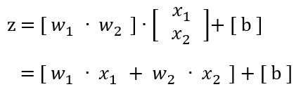
สมมติว่า X, W และ B มีค่าดังใน ภาพที่ 1 หาค่า z ได้เท่ากับ 0.36

z = [ (w1· x1 + w2· x2) + b] 
  = [0.2· 0.05 + 0.5 · 0.1] + [0.3] 
  = 0.36

Sigmoid Function

Sigmoid เป็นฟังก์ชันที่เปลี่ยนค่าทั้งหมดบนเส้นจำนวนให้กลายเป็นช่วง (0, 1) สมการคือ

sigmoid(z) = 1/(1+e^(-z))

เรียกฟังก์ชันสำหรับการปรับค่าอย่างนี้ว่า Activate Function

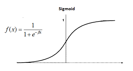
ดังนั้นผลลัพธ์สุดท้ายที่เป็นค่าที่ Model ทำนายออกมาได้ หรือ y_hat จะเท่ากับ Sigmoid(z)

def sigmoid(z):
    return 1.0/(1+ np.exp(-z))
y_hat = Sigmoid(z) 
      = Sigmoid(0.36) 
      = 0.5890

Loss Function

การคำนวน Error ว่า y hat ที่โมเดลทำนายออกมา ตรงกับ y target หรือไม่ ด้วย Loss Function (L) = Loss(y, y^) โดยที่ L อาจจะเป็น MSE (Mean Squared Error)

L = (y - y^)^2

สมมติว่า y เท่ากับ 0.7 และ L มีค่าเท่ากับ 0.0123

L = (y - y^)^2 
  = (0.7 - 0.589)^2 
  = 0.0123

Back-propagation

เมื่อได้ค่าจาก loss function แล้ว จะนำมาหา Gradient(ความชัน) ของ Loss ขึ้นกับ Weight ต่าง ๆ ทำให้ Loss น้อยลง ในการ train รอบถัดไป

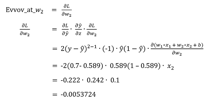
เราสามารถทำกระบวนการ Forward Propagation เพื่อปรับค่า w2 จากการหาอนุพันธ์ของ L เทียบกับ w2 หรือความชัน (Gradient) ของ Loss(y, y^) หรือ Error ที่ w2 ด้วยสมการด้านล่าง

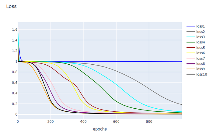
กำหนดให้ Learning Rate ตั้งแต่ 0.1, 0.2, …, 1.0 แต่ละค่า Train 1,000 Epoch ปรับค่า w2

• ถ้า Learning Rate มีค่าน้อย Weight ของโมเดลก็จะเปลี่ยนแปลงน้อย การทำงานของโมเดลก็จะเปลี่ยนไปน้อย Loss จะไม่ค่อยเปลี่ยนเท่าไร
• ถ้า Learning Rate มีค่ามาก Weight ของโมเดลก็จะเปลี่ยนแปลงมาก การทำงานของโมเดลก็จะเปลี่ยนไปมาก Loss จะเปลี่ยนแปลงมาก

#ในที่นี้ยกตัวอย่าง กำหนดให้ Learning Rate = 0.5
Update w2 = w2 - Learning_Rate*Error_at_w2 
          = 0.5 -(0.5)(-0.0053724)
          = 0.5026862

Workshop

import numpy as np

def sigmoid(x):
    return 1.0/(1+ np.exp(-x))

def sigmoid_derivative(x):
    return x * (1.0 - x)

class NeuralNetwork:
    def __init__(self, x, y, l):
        self.input      = x
        self.weights1   = np.random.rand(self.input.shape[1],4) 
        self.weights2   = np.random.rand(4,1)                 
        self.y          = y
        self.output     = np.zeros(self.y.shape)
        self.learning_rate = l
        
    def loss(self):
        return sum((self.y - self.output)**2)

    def feedforward(self):
        self.layer1 = sigmoid(np.dot(self.input, self.weights1))
        self.output = sigmoid(np.dot(self.layer1, self.weights2))

    def backprop(self): 
        d_weights2 = np.dot(self.layer1.T, (2*(self.y - self.output) * sigmoid_derivative(self.output)))
        d_weights1 = np.dot(self.input.T,  (np.dot(2*(self.y - self.output) * sigmoid_derivative(self.output), self.weights2.T) * sigmoid_derivative(self.layer1)))
        
        self.weights1 += learning_rate*d_weights1
        self.weights2 += learning_rate*d_weights2

Trian Model

learning_rate = 0.1 #ปรับค่าตรงนี้
nn = NeuralNetwork(X,y,learning_rate)

loss=[]

for i in range(1000):
    nn.feedforward()
    nn.backprop()
    loss.append(nn.loss())

Plot Loss

import pandas as pd
from matplotlib import pyplot as plt  
%matplotlib inline
import plotly
import plotly.graph_objs as go

import library ที่ต้องใช้

df = pd.DataFrame(loss, columns=['loss'])
df.head()

แสดงค่า loss ในการปรับ Learning Rate ในแต่ละครั้ง

plotly.offline.init_notebook_mode(connected=True)

h1 = go.Scatter(y=df['loss'], 
                    mode="lines", line=dict(
                    width=2,
                    color='blue'),
                    name="loss")

data = [h1]

layout1 = go.Layout(title='Loss',
                   xaxis=dict(title='epochs'),
                   yaxis=dict(title=''))
fig1 = go.Figure(data, layout=layout1)
plotly.offline.iplot(fig1)

output : ปรับการ Learning Rate ทั้งหมด 10 เส้น

Reference

Implement the Back-propagation Algorithm from Scratch with NumPy